
 This is the english version.
  Deutschsprachige Version auf geodesics.yukterez.net
● Field equation and geodesic solver:
- Code: Alles auswählen
(* |||||||||||||||||||||||||||||||||||||||||||||||||||||||||||||||||||||||||||||||||||||| *)
(*  Mathematica Syntax | EINSTEIN-MAXWELL TENSOR+GEODESIC SOLVER | geodesics.yukterez.net *)
(* |||||||||||||||||||||||||||||||||||||||||||||||||||||||||||||||||||||||||||||||||||||| *)

ClearAll["Local`*"]; LaunchKernels[4];
smp[y_]:=Simplify[y, Reals];
list[y_]:=y[[1]]==y[[2]];
rplc[y_]:=(((((((y/.t->t[τ])/.r->r[τ])/.θ->θ[τ])/.φ->φ[τ])/.Derivative[1][t[τ]]->
t'[τ])/.Derivative[1][r[τ]]->r'[τ])/.Derivative[1][θ[τ]]->θ'[τ])/.Derivative[1][φ[τ]]->φ'[τ]

                                                      (* kovariante metrische Komponenten *)
g11=gtt=-((-Δ+ж a^2 Sin[θ]^2)/(Σ χ^2));
g22=grr=-Σ/Δ;
g33=gθθ=-Σ/ж;
g44=gφφ=-((ж σ^2 Sin[θ]^2-a^2 Δ Sin[θ]^4)/(Σ χ^2));
g14=gtφ=-(( a (Δ-ж σ) Sin[θ]^2)/(Σ χ^2));
g12=g13=g23=g24=g34=0;

                                                                           (* Abkürzungen *)
Σ=r^2+a^2 Cos[θ]^2;
Δ=(r^2+a^2)(1-Λ/3 r^2)-2 M r+℧^2;
Χ=(r^2+a^2)^2-a^2 Sin[θ]^2 Δ;
щ=(q ℧ r (a^2+r^2))/(Δ Σ);
χ=1+Λ/3 a^2;
ж=1+Λ/3 a^2 Cos[θ]^2;
σ=a^2+r^2;

                           (* Dimensionen, elektrische Ladung, Spin, Vakuumenergie, Masse *)
x={t, r, θ, φ}; n=4; Ω=℧; ℧=℧; a=a; Λ=Λ; M=1;

                                                                         "Metrischer Tensor"
mt=smp[{
{g11, g12, g13, g14},
{g12, g22, g23, g24},
{g13, g23, g33, g34},
{g14, g24, g34, g44}
}];
Subscript["g", μσ] -> MatrixForm[mt]
it=smp[Inverse[mt]];
"g"^μσ -> MatrixForm[it]
mx=Table[smp[Sum[
it[[i, k]] mt[[k, j]], {k, 1, n}]],
{i, 1, n}, {j, 1, n}];
Subsuperscript["g", "μ", "σ"] -> MatrixForm[mx]
md=Det[mt]; "|g|" -> smp[md]

                                                       "Elektromagnetisches Vektorpotential"
A={Ω r/Σ/χ, 0, 0, -Ω r/Σ/χ Sin[θ]^2 a}; Subscript["A", μ]->smp[A]

                                                                            "Maxwell Tensor"
F=ParallelTable[smp[((D[A[[j]], x[[k]]]-D[A[[k]], x[[j]]]))], {j, 1, n}, {k, 1, n}];
Subscript["F", μσ] -> MatrixForm[F]
f=smp[ParallelTable[Sum[
it[[i, k]] it[[j, l]] F[[k, l]],
{k, 1, n}, {l, 1, n}], {i, 1, n}, {j, 1, n}]];
"F"^μσ -> MatrixForm[f]
џ=ParallelTable[smp[Sum[
it[[i, k]] F[[k, j]], {k, 1, n}]],
{i, 1, n}, {j, 1, n}];
Subsuperscript["F", "μ", "σ"] -> MatrixForm[џ]

                                                                        "Christoffelsymbole"
chr=ParallelTable[smp[(1/2)Sum[(it[[i, s]])
(D[mt[[s, j]], x[[k]]]+D[mt[[s, k]], x[[j]]] -D[mt[[j, k]], x[[s]]]), {s, 1, n}]],
{i, 1, n}, {j, 1, n}, {k, 1, n}];
crs=ParallelTable[If[UnsameQ[chr[[i, j, k]], 0],
{Subsuperscript["Γ", ToString[j] <> ToString[k], i] -> chr[[i, j, k]]}],
{i, 1, n}, {j, 1, n}, {k, 1, j}];
TableForm[DeleteCases[Flatten[crs], Null]]

                                                                 "gemischter Riemann Tensor"
rmn=ParallelTable[smp[
D[chr[[i, j, l]], x[[k]]] - D[chr[[i, j, k]], x[[l]]] +
Sum[chr[[s, j, l]] chr[[i, k, s]] -
chr[[s, j, k]] chr[[i, l, s]],
{s, 1, n}]], {i, 1, n}, {j, 1, n}, {k, 1, n}, {l, 1, n}];
rie=ParallelTable[If[UnsameQ[rmn[[i, j, k, l]], 0],
{Subsuperscript["R", ToString[j] <> ToString[k] <> ToString[l], i] -> rmn[[i, j, k, l]]}],
{i, 1, n}, {j, 1, n}, {k, 1, n}, {l, 1, k - 1}];
TableForm[DeleteCases[Flatten[rie], Null]]
                                                            (* kovarianter Riemann Tensor *)
rcv=ParallelTable[Sum[mt[[i, j]] rmn[[j, k, l, m]], {j, 1, n}],
{i, 1, n}, {k, 1, n}, {l, 1, n}, {m, 1, n}];
                                                        (* kontravarianter Riemann Tensor *)
rcn=ParallelTable[Sum[it[[m, i]] it[[h, j]] it[[o, k]] it[[p, l]] rcv[[i, j, k, l]],
{i, 1, n}, {j, 1, n}, {k, 1, n}, {l, 1, n}],
{m, 1, n}, {h, 1, n}, {o, 1, n}, {p, 1, n}];

                                                                              "Ricci Tensor"
rcc=ParallelTable[smp[
Sum[rmn[[i, j, i, l]], {i, 1, n}]], {j, 1, n}, {l, 1, n}];
Subscript["Ř", μσ] -> MatrixForm[rcc]
ric=ParallelTable[smp[Sum[
it[[i, k]] it[[j, l]] rcc[[k, l]], {k, 1, n}, {l, 1, n}]],
{i, 1, n}, {j, 1, n}];
"Ř"^μσ -> MatrixForm[ric]
rck=ParallelTable[smp[Sum[
it[[i, k]] rcc[[k, j]], {k, 1, n}]],
{i, 1, n}, {j, 1, n}];
Subsuperscript["Ř", "μ", "σ"] -> MatrixForm[rck]

                                                                              "Ricci Skalar"
Ř=smp[ParallelSum[it[[i, j]] rcc[[i, j]], {i, 1, n}, {j, 1, n}]]; "Ř"->Ř

                                                                        "Kretschmann Skalar"
krn= smp[ParallelSum[rcv[[i, j, k, l]] rcn[[i, j, k, l]],
{i, 1, n}, {j, 1, n}, {k, 1, n}, {l, 1, n}]];
"K"->krn

                                                                               "Weyl Tensor"
weyl1=smp[ParallelTable[
 rcv[[i, j, k, l]] -
(rcc[[i, k]] mt[[j, l]] -
 rcc[[i, l]] mt[[j, k]] +
 rcc[[j, l]] mt[[i, k]] -
 rcc[[j, k]] mt[[i, l]])/2 +
(mt[[i, k]] mt[[j, l]] -
 mt[[i, l]] mt[[j, k]])/6 Ř,
{i, 1, n}, {j, 1, n}, {k, 1, n}, {l, 1, n}]];
Weyl1=ParallelTable[If[UnsameQ[weyl1[[i, j, k, l]], 0],
{Subscript["W",
ToString[i] <> ToString[j] <> ToString[k] <> ToString[l]] -> weyl1[[i, j, k, l]]}],
{i, 1, n}, {j, 1, n}, {k, 1, n}, {l, 1, n}];
weyl2=smp[ParallelTable[
Sum[it[[m, i]] it[[h, j]] it[[o, k]] it[[p, l]] weyl1[[i, j, k, l]],
{i, 1, n}, {j, 1, n}, {k, 1, n}, {l, 1, n}],
{m, 1, n}, {h, 1, n}, {o, 1, n}, {p, 1, n}]];
Weyl2=ParallelTable[If[UnsameQ[weyl2[[i, j, k, l]], 0],
{"W"^(ToString[i] <> ToString[j] <> ToString[k] <> ToString[l]) -> weyl2[[i, j, k, l]]}],
{i, 1, n}, {j, 1, n}, {k, 1, n}, {l, 1, n}];
weyl3=ParallelTable[smp[Sum[
it[[i, m]] weyl1[[m, j, k, l]], {m, 1, n}]],
{i, 1, n}, {j, 1, n}, {k, 1, n}, {l, 1, n}];
Weyl3=ParallelTable[If[UnsameQ[weyl3[[i, j, k, l]], 0],
{Subsuperscript["W", ToString[j] <> ToString[k] <> ToString[l], ToString[i]] ->
weyl3[[i, j, k, l]]}],
{i, 1, n}, {j, 1, n}, {k, 1, n}, {l, 1, n}];
TableForm[DeleteCases[Flatten[Weyl3], Null]]

                                                                 "kontrahierter Weyl Tensor"
weyl4=ParallelTable[smp[
Sum[weyl3[[i, j, i, l]], {i, 1, n}]], {j, 1, n}, {l, 1, n}];
Subscript["Ŵ", μσ] -> MatrixForm[weyl4]
weyl5=ParallelTable[smp[Sum[
it[[i, k]] it[[j, l]] weyl4[[k, l]], {k, 1, n}, {l, 1, n}]],
{i, 1, n}, {j, 1, n}];
"Ŵ"^μσ -> MatrixForm[weyl5]
weyl6=ParallelTable[smp[Sum[
it[[i, k]] weyl4[[k, j]], {k, 1, n}]],
{i, 1, n}, {j, 1, n}];
Subsuperscript["Ŵ", "μ", "σ"] -> MatrixForm[weyl6]

                                                                               "Weyl Skalar"
Ŵ=smp[ParallelSum[it[[i, j]] rcc[[i, j]], {i, 1, n}, {j, 1, n}]]; "Ŵ"->Ŵ

                                                                           "Einstein Tensor"
est=smp[rcc-Ř mt/2];
Subscript["G", μσ] -> MatrixForm[est]
ein=ParallelTable[smp[Sum[
it[[i, k]] it[[j, l]] est[[k, l]], {k, 1, n}, {l, 1, n}]],
{i, 1, n}, {j, 1, n}];
"G"^μσ -> MatrixForm[ein]
esm=ParallelTable[smp[Sum[
it[[i, k]] est[[k, j]], {k, 1, n}]],
{i, 1, n}, {j, 1, n}];
Subsuperscript["G", "μ", "σ"] -> MatrixForm[esm]

                                                              "Stress Energie Impuls Tensor"
set=smp[(est (* -Λ mt *) )/8/π];
Subscript["T", μσ] -> MatrixForm[set]
sei=ParallelTable[smp[Sum[
it[[i, k]] it[[j, l]] set[[k, l]], {k, 1, n}, {l, 1, n}]],
{i, 1, n}, {j, 1, n}];
"T"^μσ -> MatrixForm[sei]
sem=ParallelTable[smp[Sum[
it[[i, k]] set[[k, j]], {k, 1, n}]],
{i, 1, n}, {j, 1, n}];
Subsuperscript["T", "μ", "σ"] -> MatrixForm[sem]
Ť = smp[Sum[it[[i, j]] set[[i, j]], {i, 1, n}, {j, 1, n}]]; "T" -> Ť

                                                                      "Bewegungsgleichungen"
geo=ParallelTable[smp[-Sum[
chr[[i, j, k]] x[[j]]' x[[k]]'+q f[[i, k]] x[[j]]' mt[[j, k]],
{j, 1, n}, {k, 1, n}]], {i, 1, n}];

equ=ParallelTable[{x[[i]]''[τ]==smp[rplc[geo[[i]]]]}, {i, 1, n}];

geodesic1=equ[[1]][[1]]
geodesic2=equ[[2]][[1]]
geodesic3=equ[[3]][[1]]
geodesic4=equ[[4]][[1]]

                                                                     "totale Zeitdilatation"
zd=Sum[mt[[μ, ν]] x[[μ]]' x[[ν]]', {μ, 1, n}, {ν, 1, n}];
ṫ=Quiet[rplc[smp[Normal[Solve[
-μ==(zd/.t'->ť), ť]]]]];
Derivative[1][s][τ]^2 == "ds²/dτ² == -μ" == smp[rplc[zd]]
Derivative[1][t][τ]->ṫ[[1, 1, 2]]||ṫ[[2, 1, 2]]||rplc[Sqrt[it[[1, 1]]]]/Sqrt[1-μ^2 v[τ]^2]

                                                                  "kovarianter Viererimpuls"
p[μ_]:=-(Sum[mt[[μ, ν]]*x[[ν]]', {ν, 1, n}]+q A[[μ]]);
pt[τ]->rplc[smp[p[1]]]
pr[τ]->rplc[smp[p[2]]]
pθ[τ]->rplc[smp[p[3]]]
pφ[τ]->rplc[smp[p[4]]]

                                                                       "linearer 3er-Impuls"
ṕ[i_]:=rplc[smp[Sqrt[-Sum[mt[[i, k]] x[[i]]' x[[k]]',
{k, 1, n}]]]]-Sqrt[1-μ^2 v[τ]^2] q A[[i]];
ṕr[τ]->ṕ[2]
ṕθ[τ]->ṕ[3]
ṕφ[τ]->ṕ[4]

                                                                    "lokale Geschwindigkeit"
V[x_]:=smp[Normal[Solve[vx Sqrt[-mt[[x, x]]]/Sqrt[1-μ^2 v[τ]^2]-(1-μ^2 v[τ]^2) q A[[x]]==
p[x], vx]][[1, 1]]];
rplc[V[2]]/.vx->vr[τ]
rplc[V[3]]/.vx->vθ[τ]
rplc[V[4]]/.vx->vφ[τ]
- Code: Alles auswählen
(* |||||||||||||||||||||||||||||||||||||||||||||||||||||||||||||||||||||||||||||||||||||| *)
(*  Mathematica Syntax | EINSTEIN-MAXWELL TENSOR+GEODESIC SOLVER | geodesics.yukterez.net *)
(* |||||||||||||||||||||||||||||||||||||||||||||||||||||||||||||||||||||||||||||||||||||| *)

ClearAll["Local`*"]; LaunchKernels[4];
smp[y_]:=Simplify[y,
X\[Element]Reals&&Y\[Element]Reals&&Z\[Element]Reals&&a\[Element]Reals];
list[y_]:=y[[1]]==y[[2]];
rplc[y_]:=(((((((y/.t->t[τ])/.X->X[τ])/.Y->Y[τ])/.Z->Z[τ])/.Derivative[1][t[τ]]->
t'[τ])/.Derivative[1][X[τ]]->X'[τ])/.Derivative[1][Y[τ]]->Y'[τ])/.Derivative[1][Z[τ]]->Z'[τ]

                                                      (* kovariante metrische Komponenten *)
g11=gtt=(a^2 Z^2+r^2 (-2 M r+r^2+℧^2))/(r^4+a^2 Z^2);
g22=gXX=-((a^4 r^4+2 a^2 r^6+r^8+2 M r^5 X^2+4 a M r^4 X Y+2 a^2 M r^3 Y^2+a^6 Z^2+
2 a^4 r^2 Z^2+a^2 r^4 Z^2-r^2 (r X+a Y)^2 ℧^2)/((a^2+r^2)^2 (r^4+a^2 Z^2)));
g33=gYY=-((a^4 r^4+2 a^2 r^6+r^8+2 a^2 M r^3 X^2-4 a M r^4 X Y+2 M r^5 Y^2+a^6 Z^2+
2 a^4 r^2 Z^2+a^2 r^4 Z^2-r^2 (a X-r Y)^2 ℧^2)/((a^2+r^2)^2 (r^4+a^2 Z^2)));
g44=gZZ=-((r^4+2 M r Z^2+Z^2 (a-℧) (a+℧))/(r^4+a^2 Z^2));
g12=gtX=-((r^2 (r X+a Y) (2 M r-℧^2))/((a^2+r^2) (r^4+a^2 Z^2)));
g13=gtY=(r^2 (a X-r Y) (2 M r-℧^2))/((a^2+r^2) (r^4+a^2 Z^2));
g14=gtZ=(r Z (-2 M r+℧^2))/(r^4+a^2 Z^2);
g23=gXY=(r^2 (r X+a Y) (a X-r Y) (2 M r-℧^2))/((a^2+r^2)^2 (r^4+a^2 Z^2));
g24=gXZ=-((r (r X+a Y) Z (2 M r-℧^2))/((a^2+r^2) (r^4+a^2 Z^2)));
g34=gYZ=(r (a X-r Y) Z (2 M r-℧^2))/((a^2+r^2) (r^4+a^2 Z^2));

                           (* Dimensionen, elektrische Ladung, Spin, Vakuumenergie, Masse *)
x={t, X, Y, Z}; n=4; Ω=℧; ℧=0; a=0; Λ=0; M=0;

                                                                         "Metrischer Tensor"
mt=smp[{
{g11, g12, g13, g14},
{g12, g22, g23, g24},
{g13, g23, g33, g34},
{g14, g24, g34, g44}
}];
Subscript["g", μσ] -> MatrixForm[mt]
it=smp[Inverse[mt]];
"g"^μσ -> MatrixForm[it]
mx=Table[smp[Sum[
it[[i, k]] mt[[k, j]], {k, 1, n}]],
{i, 1, n}, {j, 1, n}];
Subsuperscript["g", "μ", "σ"] -> MatrixForm[mx]
md=Det[mt]; "|g|" -> smp[md]

                                                                  "r als Funktion von X,Y,Z"
r=smp[Sqrt[-a^2+X^2+Y^2+Z^2+Sqrt[(a^2-X^2-Y^2-Z^2)^2+4 a^2 Z^2]]/Sqrt[2]]; "r"->r


                                                       "Elektromagnetisches Vektorpotential"
A=℧ r^3/(r^4+a^2+Z^2){1,(r X+a Y)/(r^2+a^2),(r Y-a Z)/(r^2+a^2),Z/r};
Subscript["A", μ]->smp[A]

                                                                            "Maxwell Tensor"
F=ParallelTable[smp[((D[A[[j]], x[[k]]]-D[A[[k]], x[[j]]]))], {j, 1, n}, {k, 1, n}];
Subscript["F", μσ] -> MatrixForm[F]
f=smp[ParallelTable[Sum[
it[[i, k]] it[[j, l]] F[[k, l]],
{k, 1, n}, {l, 1, n}], {i, 1, n}, {j, 1, n}]];
"F"^μσ -> MatrixForm[f]
џ=ParallelTable[smp[Sum[
it[[i, k]] F[[k, j]], {k, 1, n}]],
{i, 1, n}, {j, 1, n}];
Subsuperscript["F", "μ", "σ"] -> MatrixForm[џ]

                                                                        "Christoffelsymbole"
chr=ParallelTable[smp[(1/2)Sum[(it[[i, s]])
(D[mt[[s, j]], x[[k]]]+D[mt[[s, k]], x[[j]]] -D[mt[[j, k]], x[[s]]]), {s, 1, n}]],
{i, 1, n}, {j, 1, n}, {k, 1, n}];
crs=ParallelTable[If[UnsameQ[chr[[i, j, k]], 0],
{Subsuperscript["Γ", ToString[j] <> ToString[k], i] -> chr[[i, j, k]]}],
{i, 1, n}, {j, 1, n}, {k, 1, j}];
TableForm[DeleteCases[Flatten[crs], Null]]

                                                                 "gemischter Riemann Tensor"
rmn=ParallelTable[smp[
D[chr[[i, j, l]], x[[k]]] - D[chr[[i, j, k]], x[[l]]] +
Sum[chr[[s, j, l]] chr[[i, k, s]] -
chr[[s, j, k]] chr[[i, l, s]],
{s, 1, n}]], {i, 1, n}, {j, 1, n}, {k, 1, n}, {l, 1, n}];
rie=ParallelTable[If[UnsameQ[rmn[[i, j, k, l]], 0],
{Subsuperscript["R", ToString[j] <> ToString[k] <> ToString[l], i] -> rmn[[i, j, k, l]]}],
{i, 1, n}, {j, 1, n}, {k, 1, n}, {l, 1, k - 1}];
TableForm[DeleteCases[Flatten[rie], Null]]
                                                            (* kovarianter Riemann Tensor *)
rcv=ParallelTable[Sum[mt[[i, j]] rmn[[j, k, l, m]], {j, 1, n}],
{i, 1, n}, {k, 1, n}, {l, 1, n}, {m, 1, n}];
                                                        (* kontravarianter Riemann Tensor *)
rcn=ParallelTable[Sum[it[[m, i]] it[[h, j]] it[[o, k]] it[[p, l]] rcv[[i, j, k, l]],
{i, 1, n}, {j, 1, n}, {k, 1, n}, {l, 1, n}],
{m, 1, n}, {h, 1, n}, {o, 1, n}, {p, 1, n}];

                                                                              "Ricci Tensor"
rcc=ParallelTable[smp[
Sum[rmn[[i, j, i, l]], {i, 1, n}]], {j, 1, n}, {l, 1, n}];
Subscript["Ř", μσ] -> MatrixForm[rcc]
ric=ParallelTable[smp[Sum[
it[[i, k]] it[[j, l]] rcc[[k, l]], {k, 1, n}, {l, 1, n}]],
{i, 1, n}, {j, 1, n}];
"Ř"^μσ -> MatrixForm[ric]
rck=ParallelTable[smp[Sum[
it[[i, k]] rcc[[k, j]], {k, 1, n}]],
{i, 1, n}, {j, 1, n}];
Subsuperscript["Ř", "μ", "σ"] -> MatrixForm[rck]

                                                                              "Ricci Skalar"
Ř=smp[ParallelSum[it[[i, j]] rcc[[i, j]], {i, 1, n}, {j, 1, n}]]; "Ř"->Ř

                                                                        "Kretschmann Skalar"
krn= smp[ParallelSum[rcv[[i, j, k, l]] rcn[[i, j, k, l]],
{i, 1, n}, {j, 1, n}, {k, 1, n}, {l, 1, n}]];
"K"->krn

                                                                               "Weyl Tensor"
weyl1=smp[ParallelTable[
 rcv[[i, j, k, l]] -
(rcc[[i, k]] mt[[j, l]] -
 rcc[[i, l]] mt[[j, k]] +
 rcc[[j, l]] mt[[i, k]] -
 rcc[[j, k]] mt[[i, l]])/2 +
(mt[[i, k]] mt[[j, l]] -
 mt[[i, l]] mt[[j, k]])/6 Ř,
{i, 1, n}, {j, 1, n}, {k, 1, n}, {l, 1, n}]];
Weyl1=ParallelTable[If[UnsameQ[weyl1[[i, j, k, l]], 0],
{Subscript["W",
ToString[i] <> ToString[j] <> ToString[k] <> ToString[l]] -> weyl1[[i, j, k, l]]}],
{i, 1, n}, {j, 1, n}, {k, 1, n}, {l, 1, n}];
weyl2=smp[ParallelTable[
Sum[it[[m, i]] it[[h, j]] it[[o, k]] it[[p, l]] weyl1[[i, j, k, l]],
{i, 1, n}, {j, 1, n}, {k, 1, n}, {l, 1, n}],
{m, 1, n}, {h, 1, n}, {o, 1, n}, {p, 1, n}]];
Weyl2=ParallelTable[If[UnsameQ[weyl2[[i, j, k, l]], 0],
{"W"^(ToString[i] <> ToString[j] <> ToString[k] <> ToString[l]) -> weyl2[[i, j, k, l]]}],
{i, 1, n}, {j, 1, n}, {k, 1, n}, {l, 1, n}];
weyl3=ParallelTable[smp[Sum[
it[[i, m]] weyl1[[m, j, k, l]], {m, 1, n}]],
{i, 1, n}, {j, 1, n}, {k, 1, n}, {l, 1, n}];
Weyl3=ParallelTable[If[UnsameQ[weyl3[[i, j, k, l]], 0],
{Subsuperscript["W", ToString[j] <> ToString[k] <> ToString[l], ToString[i]] ->
weyl3[[i, j, k, l]]}],
{i, 1, n}, {j, 1, n}, {k, 1, n}, {l, 1, n}];
TableForm[DeleteCases[Flatten[Weyl3], Null]]

                                                                 "kontrahierter Weyl Tensor"
weyl4=ParallelTable[smp[
Sum[weyl3[[i, j, i, l]], {i, 1, n}]], {j, 1, n}, {l, 1, n}];
Subscript["Ŵ", μσ] -> MatrixForm[weyl4]
weyl5=ParallelTable[smp[Sum[
it[[i, k]] it[[j, l]] weyl4[[k, l]], {k, 1, n}, {l, 1, n}]],
{i, 1, n}, {j, 1, n}];
"Ŵ"^μσ -> MatrixForm[weyl5]
weyl6=ParallelTable[smp[Sum[
it[[i, k]] weyl4[[k, j]], {k, 1, n}]],
{i, 1, n}, {j, 1, n}];
Subsuperscript["Ŵ", "μ", "σ"] -> MatrixForm[weyl6]

                                                                               "Weyl Skalar"
Ŵ=smp[ParallelSum[it[[i, j]] rcc[[i, j]], {i, 1, n}, {j, 1, n}]]; "Ŵ"->Ŵ

                                                                           "Einstein Tensor"
est=smp[rcc-Ř mt/2];
Subscript["G", μσ] -> MatrixForm[est]
ein=ParallelTable[smp[Sum[
it[[i, k]] it[[j, l]] est[[k, l]], {k, 1, n}, {l, 1, n}]],
{i, 1, n}, {j, 1, n}];
"G"^μσ -> MatrixForm[ein]
esm=ParallelTable[smp[Sum[
it[[i, k]] est[[k, j]], {k, 1, n}]],
{i, 1, n}, {j, 1, n}];
Subsuperscript["G", "μ", "σ"] -> MatrixForm[esm]

                                                              "Stress Energie Impuls Tensor"
set=smp[(est (* -Λ mt *) )/8/π];
Subscript["T", μσ] -> MatrixForm[set]
sei=ParallelTable[smp[Sum[
it[[i, k]] it[[j, l]] set[[k, l]], {k, 1, n}, {l, 1, n}]],
{i, 1, n}, {j, 1, n}];
"T"^μσ -> MatrixForm[sei]
sem=ParallelTable[smp[Sum[
it[[i, k]] set[[k, j]], {k, 1, n}]],
{i, 1, n}, {j, 1, n}];
Subsuperscript["T", "μ", "σ"] -> MatrixForm[sem]
Ť = smp[Sum[it[[i, j]] set[[i, j]], {i, 1, n}, {j, 1, n}]]; "T" -> Ť

                                                                      "Bewegungsgleichungen"
geo=ParallelTable[smp[-Sum[
chr[[i, j, k]] x[[j]]' x[[k]]'+q f[[i, k]] x[[j]]' mt[[j, k]],
{j, 1, n}, {k, 1, n}]], {i, 1, n}];

equ=ParallelTable[{x[[i]]''[τ]==smp[rplc[geo[[i]]]]}, {i, 1, n}];

geodesic1=equ[[1]][[1]]
geodesic2=equ[[2]][[1]]
geodesic3=equ[[3]][[1]]
geodesic4=equ[[4]][[1]]

                                                                     "totale Zeitdilatation"
zd=Sum[mt[[μ, ν]] x[[μ]]' x[[ν]]', {μ, 1, n}, {ν, 1, n}];
ṫ=Quiet[rplc[smp[Normal[Solve[
-μ==(zd/.t'->ť), ť]]]]];
Derivative[1][s][τ]^2 == "ds²/dτ² == -μ" == smp[rplc[zd]]
Derivative[1][t][τ]->ṫ[[1, 1, 2]]||ṫ[[2, 1, 2]]||rplc[Sqrt[it[[1, 1]]]]/Sqrt[1-μ^2 v[τ]^2]

                                                                  "kovarianter Viererimpuls"
p[μ_]:=-(Sum[mt[[μ, ν]]*x[[ν]]', {ν, 1, n}]+q A[[μ]]);
pt[τ]->rplc[smp[p[1]]]
pX[τ]->rplc[smp[p[2]]]
pY[τ]->rplc[smp[p[3]]]
pZ[τ]->rplc[smp[p[4]]]

                                                                       "linearer 3er-Impuls"
ṕ[i_]:=rplc[smp[Sqrt[-Sum[mt[[i, k]] x[[i]]' x[[k]]',
{k, 1, n}]]]]-Sqrt[1-μ^2 v[τ]^2] q A[[i]];
ṕX[τ]->ṕ[2]
ṕY[τ]->ṕ[3]
ṕZ[τ]->ṕ[4]

                                                                    "lokale Geschwindigkeit"
V[x_]:=smp[Normal[Solve[vx Sqrt[-mt[[x, x]]]/Sqrt[1-μ^2 v[τ]^2]-(1-μ^2 v[τ]^2) q A[[x]]==
p[x], vx]][[1, 1]]]; ν[i_]:=rplc[smp[Sqrt[-Sum[mt[[i, k]] x[[i]]' x[[k]]', {k, 1, n}]]]]/γ;
rplc[V[2]]/.vx->vX[τ]
rplc[V[3]]/.vx->vY[τ]
rplc[V[4]]/.vx->vZ[τ]
 The upper solver is by default set to the KNdS-metric in {t,r,θ,φ}-BL-coordinates. With Λ=0 the metric reduces to Kerr Newman, with Λ=℧=0 to Kerr, with Λ=a=0 to Reissner Nordström, with Λ=℧=a=0 to Schwarzschild, with ℧=a=0 to Schwarzschild De Sitter, with ℧=a=M=0 to De Sitter and with Λ=℧=a=M=0 to Minkowski. The lower solver is set to Kerr Newman in cartesian coordinates (since the metric is more complicated this way that needs takes more time to solve). If the line element is given in a cumbersome form the metric coefficients can be extracted with the line element decomposer.
● Examples of various metrics in different coordinates:
Boyer Lindquist is the rotating equivalent to Droste (time coordinate of a field free and stationary observer), Kerr-Schild to Finkelstein (the time coordinate will be stamped by infalling light rays) and Doran to Raindrop coordinates (the proper time of free falling clocks stamp the coordinate time). In the equations of motion the coordinates become functions of the proper time, or in case of photons of the affine parameter (t→t[τ], r'→r'[τ], θ''→θ''[τ] etc). By default natural units with G=M=c=K=1 are used (lengths are given in GM/c², time in GM/c³, velocity in c, etc). The cosmological constant in our universe has the value Λ=1.1056e-52/m², where the vacuum density is ρΛ=c²Λ/(8πG). In the context of a black hole with M=1e40kg, the cosmological constant in natural units would be Λ→G²M²Λ/c⁴=6.0963e-87.● Coordinate transformator:
- Code: Alles auswählen
(* |||||||||||||||||||||||||||||||||||||||||||||||||||||||||||||||||||||||||||||||||||||| *)
(* ||||| KOORDINATEN TRANSFORMATOR | geodesics.yukterez.net | Droste -> Finkelstein ||||| *)
(* |||||||||||||||||||||||||||||||||||||||||||||||||||||||||||||||||||||||||||||||||||||| *)

d1={dt, dr, dθ, dφ};
d2={dT, dr, dθ, dφ};
n=4;

"Schwarzschild, Droste"

g11=gtt=1-2M/r;
g22=grr=-1/gtt;
g33=gθθ=-r^2;
g44=gφφ=-r^2 Sin[θ]^2;
g12=g13=g14=g23=g24=g34=0;

m1={
{g11, g12, g13, g14},
{g12, g22, g23, g24},
{g13, g23, g33, g34},
{g14, g24, g34, g44}};

A1={0, 0, 0, 0};
Subscript["A", μ] -> A1

M1=MatrixForm[m1];
Subscript["g", μσ] -> M1

"Schwarzschild, Finkelstein"

v=-2M/r;
dt=dT+v/gtt dr ;

m2=FullSimplify[Table[Sum[D[d1[[k]], d2[[i]]] D[d1[[s]], d2[[j]]] m1[[k, s]],
{k, 1, n}, {s, 1, n}], {i, 1, n}, {j, 1, n}]];
M2=MatrixForm[m2];
Subscript["g", μσ] -> M2

A2=FullSimplify[Table[Sum[D[d1[[k]], d2[[i]]] A1[[k]],
{k, 1, n}], {i, 1, n}]];
Subscript["A", μ] -> A2


Quit[]


(* |||||||||||||||||||||||||||||||||||||||||||||||||||||||||||||||||||||||||||||||||||||| *)
(* |||| KOORDINATEN TRANSFORMATOR | geodesics.yukterez.net | Sphärisch -> Kartesisch |||| *)
(* |||||||||||||||||||||||||||||||||||||||||||||||||||||||||||||||||||||||||||||||||||||| *)

d1={dt, dr, dθ, dΦ};
d2={dt, dX, dY, dZ};
n=4;

"Schwarzschild, Droste, Sphärisch"

g11=gtt=1-2/r;
g22=gXX=-1/g11;
g33=gYY=-r^2;
g44=gZZ=-r^2 Sin[θ]^2;
g12=gtX=0;
g13=gtY=0;
g14=gtZ=0;
g23=gXY=0;
g24=gXZ=0;
g34=gYZ=0;

m1={
{g11, g12, g13, g14},
{g12, g22, g23, g24},
{g13, g23, g33, g34},
{g14, g24, g34, g44}};

M1=MatrixForm[m1];
Subscript["g", μσ] -> M1

A1={0, 0, 0, 0};
Subscript["A", μ] -> A1

"Schwarzschild, Droste, Kartesisch"

dr=(X dX+Y dY+Z dZ)/r;
dθ=(Z X dX+Z Y dY-(X^2+Y^2) dZ)/r^2/Sqrt[X^2+Y^2];
dΦ=(X dY-Y dX)/(X^2+Y^2);

r=Sqrt[X^2+Y^2+Z^2];
θ=ArcTan[Z, Sqrt[X^2+Y^2]];

m2=FullSimplify[Table[Sum[D[d1[[k]], d2[[i]]] D[d1[[s]], d2[[j]]] m1[[k, s]],
{k, 1, n}, {s, 1, n}], {i, 1, n}, {j, 1, n}]];
M2=MatrixForm[m2];
Subscript["g", μσ] -> M2

A2=FullSimplify[Table[Sum[D[d1[[k]], d2[[i]]] A1[[k]],
{k, 1, n}], {i, 1, n}]];
Subscript["A", μ] -> A2


Quit[]


(* |||||||||||||||||||||||||||||||||||||||||||||||||||||||||||||||||||||||||||||||||||||| *)
(* || KOORDINATEN TRANSFORMATOR | geodesics.yukterez.net | Boyer Lindquist -> Raindrop || *)
(* |||||||||||||||||||||||||||||||||||||||||||||||||||||||||||||||||||||||||||||||||||||| *)

d1={dt, dr, dθ, dΦ};
d2={dT, dr, dθ, dφ};
n=4;

"Kerr Newman, Boyer Lindquist"

g11=gtt=-(2r-r^2-℧^2-a^2+a^2 Sin[θ]^2)/(r^2+a^2 Cos[θ]^2);
g22=grr=-(r^2+a^2 Cos[θ]^2)/(a^2-2r+r^2+℧^2);
g33=gθθ=-r^2-a^2 Cos[θ]^2;
g44=gφφ=-((a^2+r^2)^2 Sin[θ]^2-a^2 (a^2-2r+r^2+℧^2) Sin[θ]^4)/(r^2+a^2 Cos[θ]^2);
g14=gtφ=-(a (℧^2-2r) Sin[θ]^2)/(r^2+a^2 Cos[θ]^2);
g12=g13=g23=g24=g34=0;

m1={
{g11, g12, g13, g14},
{g12, g22, g23, g24},
{g13, g23, g33, g34},
{g14, g24, g34, g44}};

M1=MatrixForm[m1];
Subscript["g", μσ] -> M1

A1={r ℧/(r^2+a^2 Cos[θ]^2), 0, 0, -a r ℧ Sin[θ]^2/(r^2+a^2 Cos[θ]^2)};
Subscript["A", μ] -> A1

"Kerr Newman, Raindrop"

σ=+a^2+r^2;
v=-Sqrt[2r-℧^2]/Sqrt[σ];
dt=+dT+v dr/(1-v^2);
dΦ=+dφ+a v dr/σ/(1-v^2);

m2=FullSimplify[Table[Sum[D[d1[[k]], d2[[i]]] D[d1[[s]], d2[[j]]] m1[[k, s]],
{k, 1, n}, {s, 1, n}], {i, 1, n}, {j, 1, n}]];
M2=MatrixForm[m2];
Subscript["g", μσ] -> M2

A2=FullSimplify[Table[Sum[D[d1[[k]], d2[[i]]] A1[[k]],
{k, 1, n}], {i, 1, n}]];
Subscript["A", μ] -> A2
Transformation from one coordinate system into an other. Input: covariant metric and transformation rule, Output: new covariant metric (for an example see below).● Example for the coordinate transformation:
Above: transformation rule, below: transformationExample, Input: Schwarzschild metric in covariant Droste Bookkeeper coordinates (left) and the transformation rule dτ=dt-v·dr/gₜₜ, Output: Schwarzschild metric in covariant Gullstrand Painlevé (Raindrop) coordinates (right). For the backtransformation click on the image. Equivalent transformation for the Kerr Newman metric: click.● Function plotter:
- Code: Alles auswählen
(* |||||||||||||||||||||||||||||||||||||||||||||||||||||||||||||||||||||||||||||||||||||| *)
(* | Mathematica Syntax | EINSTEIN PLOTTER | geodesics.yukterez.net | Version 10.1.2020 | *)
(* |||||||||||||||||||||||||||||||||||||||||||||||||||||||||||||||||||||||||||||||||||||| *)

(* Kartesisch zu Boyer Lindquist *)
k[x_, z_, a_]:=FindInstance[x==Sqrt[R^2+a^2]Sin[u]&&z==R Cos[u]&&u<2Pi&&u>=0&&R>=0, {R, u}, Reals]
r[x_, z_, a_]:=k[x, z, a][[1, 1, 2]];
θ[x_, z_, a_]:=k[x, z, a][[1, 2, 2]];

(* Kretschmann Skalar *)
K[x_, z_, a_, ℧_]:=-(1/((a^2+a^2 Cos[2 θ[x, z, a]]+2 r[x, z, a]^2)^6))32 (30 a^6-42 a^4 ℧^4+3 a^6 Cos[6 θ[x, z, a]]+360 a^4 ℧^2 r[x, z, a]-540 a^4 r[x, z, a]^2+272 a^2 ℧^4 r[x, z, a]^2-960 a^2 ℧^2 r[x, z, a]^3+720 a^2 r[x, z, a]^4-112 ℧^4 r[x, z, a]^4+192 ℧^2 r[x, z, a]^5-96 r[x, z, a]^6+2 a^4 Cos[4 θ[x, z, a]] (9 a^2-7 ℧^4+60 ℧^2 r[x, z, a]-90 r[x, z, a]^2)+a^2 Cos[2 θ[x, z, a]] (45 a^4+16 r[x, z, a]^2 (17 ℧^4-60 ℧^2 r[x, z, a]+45 r[x, z, a]^2)-8 a^2 (7 ℧^4-60 ℧^2 r[x, z, a]+90 r[x, z, a]^2)));

(* Horizonte und Ergosphären *)
rE=1+Sqrt[1-a^2 Cos[Θ]^2-a^2];(*äußere Ergosphäre*)
RE={Sqrt[rE^2+a^2] Sin[Θ], rE Cos[Θ]};
rG=1-Sqrt[1-a^2 Cos[Θ]^2-a^2];(*innere Ergosphäre*)
RG={Sqrt[rG^2+a^2] Sin[Θ], rG Cos[Θ]};
rA=1+Sqrt[1-a^2-a^2];(*äußerer Horizont*)
RA={Sqrt[rA^2+a^2] Sin[Θ], rA Cos[Θ]};
rI=1-Sqrt[1-a^2-a^2];(*innerer Horizont*)
RI={Sqrt[rI^2+a^2] Sin[Θ], rI Cos[Θ]};

(* Kartesischer Plot *)
℧=a;
Do[Print[Rasterize[Grid[{{
Show[
ContourPlot[K[x, z, a, ℧], {x, 0, 5}, {z, 0, 5}, PlotLegends->Automatic, Contours->20, ContourShading->Automatic, MaxRecursion->3, ImageSize->400],
ParametricPlot[{RI, RA, RG, RE}, {Θ, 0, Pi/2}, Frame->False]
]}, {"a"->N@a}, {"℧"->N@℧},
{"                                                                                  "}},
Alignment->Left]]],
{a, 0, Sqrt[1/2], Sqrt[1/2]/2}]
The default setting of the plotter is a contur plot of the Kretschmann skalar for a Kerr Newman black hole. Other functions can be plugged in from the field equation solver, when projecting to the x,z-plane r,θ-coordinates must be written as explicit functions of x,z (r→r[x,z,a], θ→θ[x,z,a]).● Example for the visualization:
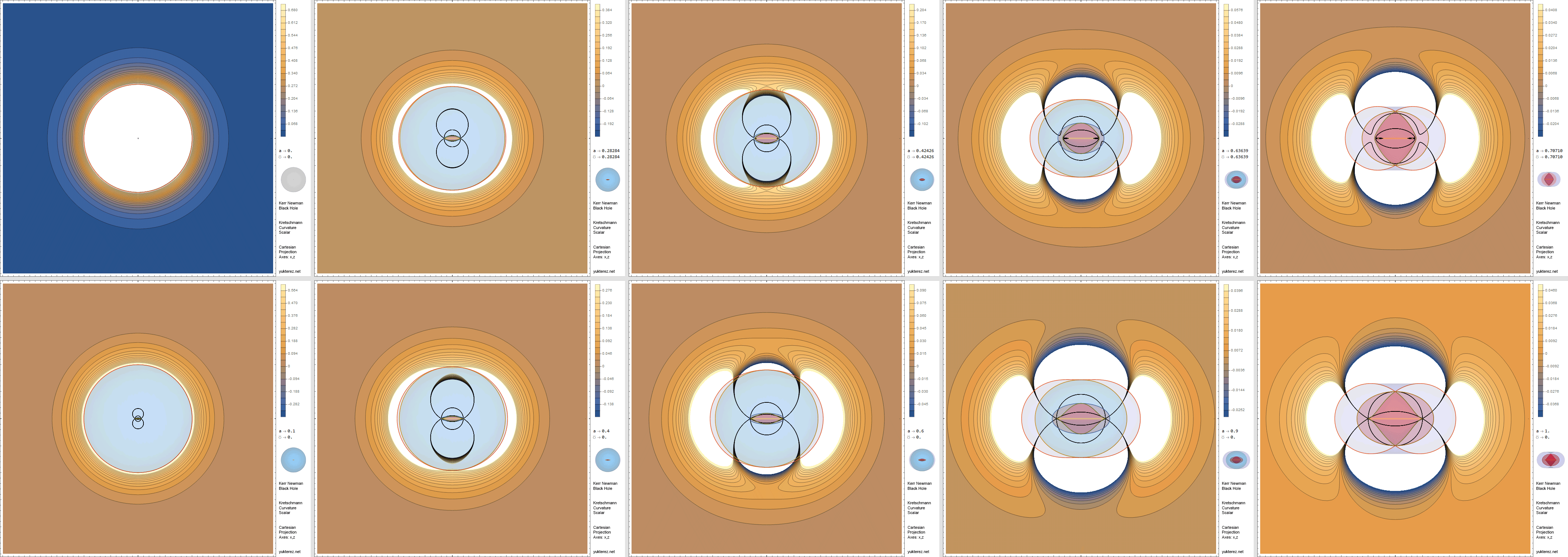 In this example the Kretschmann Skalar for a Kerr Newman BH is projected onto the x,z-plane at y=0 and overlayed with the horizons and ergospheres. The black lines mark surfaces of constant curvature; the clipped areas are marked white and have either strong positive or negative curvature. The bundled bold black lines separating the white areas mark the crossings between strong positive and negative curvature. For other spin/charge-combinations click on the image, for the animation click here.
● Equations and rules:
Field equation with respect to the covariant energy-momentum-tensor Tᵢⱼ (the gray part is not required since we treat Λ as vacuum energy density and add it to the other energy densities in the energy/momentum-tensor; if Λ is not treated as dark energy but classicaly like Einstein meant it in his so called biggest blunder, the term gets substracted as shown in gray if the signature is +---, while with -+++ it must be added in order for the cosmological constant to not show up as energy density in Tᵢⱼ):

Riemann tensor:

Ricci tensor:

Ricci scalar:

Kretschmann scalar:

Einstein tensor:

Kronecker delta:
Christoffel symbols of the 2nd kind:
Hamiltonian, for particles: μ=-1, for photons: μ=0:

Maxwell tensor and vector-potential A:

1st proper time derivatives and momentum:

Total time dilatation and local velocity:
Velocity of the local reference frames in the k-direction (relative to fixed coordinates):
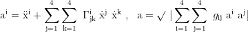
2nd proper time derivatives of a free particle:

Proper acceleration (force) for a nongeodesic particle:
Parallel transport of a vector V:
Rule for raising and lowering the indices:
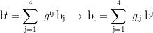
Multiple indices:
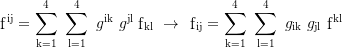
Contraction:
Mixed indices:
Transformation from one coordinate system x into an other one x̅:
In this article natural units are used. The overdot stands for differentiation by proper time τ: ẋ=dx/dτ
● Recommended tutorials:
- Text:
- Standard Reference: Bertschinger (1993)
- Standard Reference: Stefani et al (2003)
- Standard Reference: MTW (1973)
- Tutorial: Hartle (2004)
Video: - Playlist: Neil Turok (2017)
- Playlist: Paul Wagner (2018)
- Playlist: Jörn Loviscach (2016)
- Playlist: Einstein Toolkit (2017)
- Playlist: Leonard Susskind (2012)
- Playlist: Frederic Schuller (2015)
- Playlist: Eugene Khutoryansky (2017)
- Playlist: Emil Akhmenov (2016)
- Playlist: Science Clic (2020)
- Playlist: Trin Tragula (2017)
- Playlist: Eigenchris (2020)
images and animations by Simon Tyran, Vienna (Yukterez) - reuse permitted under the Creative Commons License CC BY-SA 4.0

